匈牙利匹配算法（Hungarian Matching Algorithm)，也称为 Kuhn-Munkres 算法，是一个 $O\big(|V|^3\big)$ （$V$ 表示二分图的顶点集）算法，可用于在二分图中找到最大权重匹配，有时称为分配问题。匈牙利算法被文章 End-to-End Object Detection with Transformers 中提出 DETR 算法中所采用，用于匹配预测目标框与真实目标框。除此之外，该算法也在多目标跟踪、实例分割、多人3D位姿估计等领域中发挥作用。本篇对匈牙利算法进行简单讲解。

历史

匈牙利算法是一种在多项式时间内求解任务分配问题的组合优化算法，并推动了后来的原始对偶方法。美国数学家哈罗德·库恩于 1955 年提出该算法。此算法之所以被称作匈牙利算法，是因为算法很大一部分是基于以前匈牙利数学家 Dénes Kőnig 和 Jenő Egerváry 的工作之上创建起来的。

詹姆士·芒克勒斯在 1957 年回顾了该算法，并发现（强）多项式时间的复杂度。此后该算法被称为 Kuhn–Munkres 算法或 Munkres 分配算法。原始算法的时间复杂度为 $O(|V|^4)$，但杰克·爱德蒙斯与卡普发现可以修改算法达到 $O(|V|^3)$运行时间，富泽也独立发现了这一点。L·R·福特和D·R·福尔克森将该方法推广到了一般运输问题。2006 年发现卡尔·雅可比在 19 世纪就解决了指派问题，该解法在他死后的 1890 年以拉丁文发表。

二分图

图 $G = (V, E)$ 是二分的（bipartite），如果存在一个划分使得
$$
V = X \cup Y, X \cap Y = \emptyset, E \subseteq X \times Y.
$$
这里 $V$ 是顶点集，$E$ 是边集。换句话说，就是顶点集合分成两类，每类之间的顶点没有边相连接，只有不同顶点集合的点之间才可以有边相连接。

匹配（matching）$M \subseteq E$ 是一个边集合，使得 $\forall v \in V$ 至多只属于 $M$ 中的一个边。匹配 $M$ 中边的个数称为匹配的大小，记作 $|M|$. 最大匹配（maximum matching）是一个匹配，使得任何其他匹配 $M^{\prime}$ 满足 $|M^{\prime}| \leq |M|$.

顶点 $v$ 是匹配的，如果它是匹配 $M$ 的某个边的端点，否则，称为是自由的。

如上图左图，$Y_2$, $Y_3$, $Y_4$, $Y_6$, $X_2$, $X_4$, $X_5$, $X_6$ 是匹配的，其他点是自由的。

一个边集合 $P \subseteq E$ 是道路，如果 $P$ 中的所有边都连接在一起。一个道路是交替的，如果它的边交替取自 $M$ 和 $E-M$. 如上图右图，$Y_1$, $X_2$, $Y_2$, $X_4$, $Y_4$, $X_5$, $Y_3$, $X_3$ 是交替的。

一个交替道路是增广交替道路，如果它的两个端点都是自由的。

一个匹配 $M$ 是完美匹配，如果任意的顶点都是 $M$ 中的某个边的端点。

对于加权二分图，就是每个边 $v=(i,j)$ 都分配权重值 $w(i,j)$. 匹配 $M$ 的权值是其中所有边的权值和，即
$$
w(M) = \sum_{e \in M} w(e).
$$
二分图匹配问题可以分为两种，一种是求解最大匹配，一种是求解最大权重匹配。第一种是不考虑边权重，只需要找到匹配 $M$ 使得匹配的大小 $|M|$ 最大。第二种是假设每条边的权重不是相同的，需要找到匹配 $M$ 使得匹配的权值 $w(M)$ 最大。其实，第一种可以看作是第二种的特殊情形，只需要把权重看作相同即可。因此，本篇以第二种为例进行介绍。

最大权重匹配一定是完美匹配。

一个二分图是完全的，如果两个顶点集合 $X$, $Y$ 中，任意的点 $x \in X (y \in Y)$ 都与 $y \in Y (x \in X)$ 中的点有边 $e \in E$ 相连。如果一个二分图不是完全的，可以考虑把它变成完全的，通过添加权重为 0 的边。当求解的是最大匹配问题时，添加权重为 inf 的边。

二分图可以很容易地用邻接矩阵表示，其中边的权重是矩阵元素。从邻接矩阵的角度考虑图形对于匈牙利算法很有用。

使用邻接矩阵的匈牙利算法

假设您想举办一个派对，并且您想要一位音乐家(musician)进行表演，一位厨师(chef)准备食物，以及在派对结束后进行清洁服务的清洁工(cleaner)。有 3 家公司提供这三种服务中的每一种，但一家公司一次只能提供一种服务（即 B 公司不能同时提供清洁工和厨师）。您正在决定应该从哪家公司购买每项服务，以最大限度地减少聚会的成本。你意识到这是分配问题的一个例子，并着手根据以下信息制作一个图表：

公司	音乐家	厨师	清洁工
公司 A	108	125	150
公司 B	150	135	175
公司 C	122	148	250

用二分图表示如下

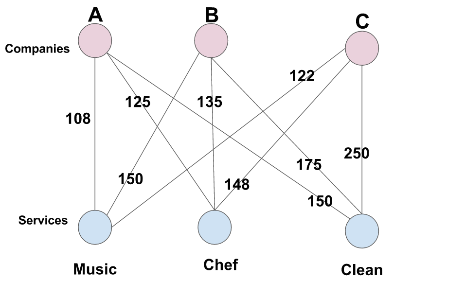
如何解决上面的最大权重匹配问题，可以考虑蛮力法，列举所有的可能组合，但是，当二分部越来越大时，这将是非常低效的。

求二分图的最大权重匹配和最小权重匹配没有什么本质区别。对于二分图，只需要把权重系数用最大的减去所有边的权重，把二分图的最大权重匹配问题转化为求最小权重匹配。当考虑权重和最小时，我们称邻接矩阵是成本矩阵(cost matrix)；当考虑权重和最大时，我们称邻接矩阵是效益矩阵(profit matrix)。

考虑到上述示例中的成本矩阵，匈牙利算法基于这一关键思想进行操作：如果在成本矩阵的任何一行或一列的所有条目中添加或减去一个数字，则为由此产生的成本矩阵也是原始成本矩阵的最佳匹配。

如下算法将最小权重匹配问题转化为 0 匹配问题。即把寻找权重和最小的匹配转化为寻找权重和等于 0 的匹配。

匈牙利方法，针对 n x n 成本矩阵。
1. 对于每一行，把所有元素减去该行中的最小元素。这将使每行中的最小元素等于 0；
2. 对于每一列，把所有元素减去该列中的最小元素（可能取到上一次行操作得到的 0）。这将使每列中的最小元素等于 0；
3. 画最少的线（行或列），使得覆盖所有的 0； 
4. 如果绘制了 n 条线，则得到了最佳的零匹配，算法完成。如果条数小于 n，则尚未达到最佳的零匹配，进入下一步； 
5. 找到未被任何线覆盖的最小元素。从未划掉的每一行中减去该元素，并将最小元素添加到划掉的每一列中（使得列中的最小元素仍然是 0 ）。然后，返回到步骤 3。

利用匈牙利算法求解上面的最小权重匹配问题。

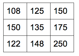
初始邻接矩阵：

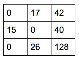
每一行减去行最小元素：

每一列减去列最小元素：

画最少的线覆盖包含 0 的行和列：

发现共有两条线，分别是第一列和第二行，而 $2 < 3$，所以，还需要继续进行约简。对没有覆盖的两行减去两行中的最小元素：

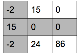
对覆盖的列加上刚刚减去的最小元素，使得列中的 0 恢复：

继续画线，用最少的线覆盖所有的 0：

画线个数 3 等于邻接矩阵的行数。所得的匹配是矩阵中的 0，它在每行和每列中只能取1个：

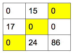
替换 0 为原始权重值：

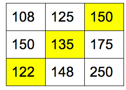
匈牙利算法告诉我们最小的花费（407 = 150 + 135 + 122）是请 A 公司的清洁工，B 公司的厨师，C 公司的音乐家。通过蛮力解法可以验证结果的正确性。

使用图的匈牙利算法

不使用邻接矩阵，直接使用二分图寻找最大权重匹配，需要对每个顶点定义标签值，称为可行标签（feasible labeling）.

A labeling for graph $G = (V, E)$ is a function $l: V \to \mathbb{R}$, such that:
$$
\forall (u, v) \in E: l(u) + l(v) \geq w(u, v).
$$
An Equality Subgraph is a subgraph $G_l = (V, E_l)$ $ \subseteq$ $G = (V, E)$, fixed on a labeling $l$, such that
$$
E_l = \lbrace(u,v) \in E: l(u) + l(v) = w(u,v)\rbrace.
$$

The Kuhn-Munkres Theorem

Given labeling $l$, if $M$ is a perfect matching on $G_l$, then $M$ is maximal-weight matching of $G$.

Let $M^{\prime}$ be any perfect matching in $G$. By definition of a labeling function and since $M^{\prime}$ is perfect,
$$
w(M^{\prime}) = \sum_{(u,v)\in M^{\prime}} w(u,v) \leq \sum_{(u,v)\in M^{\prime}} l(u) + l(v) = \sum_{v\in V} l(v).
$$
This means: $\sum_{v\in V} l(v)$ is an upper bound for any perfect matching $M^{\prime}$ of $G$.
Now look at the weight of matching $M$:
$$
w(M) = \sum_{(u,v)\in M} w(u,v) = \sum_{(u,v)\in M} l(u) + l(v) = \sum_{v\in V} l(v).
$$
we have that for all perfect matchings $M^{\prime}$ of $G$:
$$
w(M) \geq w(M^{\prime}).
$$

根据 Kuhn-Munkres 定理，找到最大权重分配的问题被简化为找到正确的标记函数和相应等价子图上的任何完美匹配。

The Hungarian Algorithm

算法思想：维护一个匹配的 $M$ 和等价图 $G_l$，从 $M = \emptyset$ 和一个有效的 $l$ 开始。继续直到 $M$ 成为 $G_l$ 上的完美匹配。每一步：要么增加 $M$ 要么改进标签 $l \to l^{\prime}$.

Augment the matching $M$

Given labeling $l$, $G_l = (V, E_l)$, some matching $M$ on $G_l$ , unmatched $u \in V, u \notin M$.

A path is augmenting for $M$ on $G_l$ if it alternates between $E_l − M$ and $M$, and the first and last vertices of the path are un-matched in $M$. Keep track of an ”almost” augmenting path starting at $u$.
If we can find an unmatched vertex $v$, then we create augmenting path $\alpha$ from $u$ to $v$.
Flip the matching by replacing the edges in $M$ with the edges in the augmenting path that are in $E_l − M$.
Since we start and end unmatched, this increases the size of the matching, $|M^{\prime}| > |M|$.

Improve the labeling $l$

$S\subseteq X$ and $T \subseteq Y$ s.t. $S,T$ represent the current “almost” augmenting alternating path between the matching $M$ and outside other edges in $E_l \to M$.
Let $N_l(S)$ be the neighbors to each node in $S$ along $E_l$.

$$
N_l(S) = \lbrace v | \forall u \in S: (u, v) \in E_l \rbrace.
$$
if $N_l(S)=T$ we cannot increase the alternating path and augment, so we must improve the labeling.
compute:
$$
\delta_l = \min_{u\in S, v \notin T} \lbrace l(u) + l(v) - w(u,v) \rbrace.
$$
improve $l \to l^{\prime}$:
$$
l^{\prime}(r) =
\begin{cases}
l(r) - \delta_l & \text{if} \ r \in S \\
l(r) + \delta_l & \text{if} \ r \in T \\
l(r) & \text{otherwise}.
\end{cases}
$$
claim: $l^{\prime}$ is a valid labeling and $E_l \subseteq E_{l^{\prime}}$.
proof follows by examining cases for all possibilities of membership of $u\in S$, $u \notin S$, $v \in T$, $v \notin T$.

the hungarian algorithm

start with some matching $M$, and a valid labeling

$$
l := \forall x \in X, y \in Y, l(y) = 0, l(x) = \max_{y^{\prime} \in Y }(w(x, y^{\prime})).
$$
do the following until $M$ is a perfect matching:

(a). Look for augmenting path;

(b). If a augmenting path does not exist, improve $l \to l^{\prime}$ and go to step (a).

Python 执行匈牙利算法

scipy.optimize.linear_sum_assignment

scipy.optimize.linear_sum_assignment(cost_matrix, maximize=False)

cost_matrix 表示代价矩阵， maximize 表示求最小（False）还是最大（True）权重匹配

from scipy.optimize import linear_sum_assignment

# 此处的 0 不是表示边缺失。表示边缺失用 np.inf 来表示
cost = np.array([[4, 1, 3], [2, 0, 5], [3, 2, 2]])
# row_ind 是排序好的，col_ind 相对应
row_ind, col_ind = linear_sum_assignment(cost)
# 表示第1，0，2列
col_ind
array([1, 0, 2])
# 最终得到完美匹配的权重和
cost[row_ind, col_ind].sum()
5

scipy.sparse.csgraph.min_weight_full_bipartite_matching

scipy.sparse.csgraph.min_weight_full_bipartite_matching(biadjacency_matrix, maximize=False)

对于稀疏矩阵进行计算。

from scipy.sparse import csr_matrix
from scipy.sparse.csgraph import min_weight_full_bipartite_matching

# 此处的 0 表示边缺失，赋值 0 将其转化为完全图
# 所以，此处就是找最大匹配
biadjacency_matrix = csr_matrix([[1, 1, 1], [1, 0, 0], [0, 1, 0]])
row_ind, col_ind = min_weight_full_bipartite_matching(biadjacency_matrix)
print(col_ind)
[2 0 1]
biadjacency_matrix[row_ind, col_ind].sum()
3

scipy.sparse.csgraph.maximum_bipartite_matching

scipy.sparse.csgraph.maximum_bipartite_matching(graph, perm_type=’row’)

from scipy.sparse import csr_matrix
from scipy.sparse.csgraph import maximum_bipartite_matching

# 此处的 0 表示边缺失，赋值 0 将其转化为完全图
# 所以，此处就是找最大匹配
graph = csr_matrix([[0, 0, 1], [1, 1, 0]])
maximum_bipartite_matching(graph, perm_type='column')
# 结果表示第0行的第2列，第1行的第0列
array([2, 0], dtype=int32)

maximum_bipartite_matching(graph, perm_type='row')
# 结果表示第0列的第1行，第1列没有，第2列的第0行
array([ 1, -1,  0], dtype=int32)